Example xymasking
XYMasking aug in Albumentations
This transform is a generalization of the TimeMasking and FrequencyMasking from torchaudio.
Python
import torchaudio
import torch
from pathlib import Path
import numpy as np
import pandas as pd
(128, 256, 4)
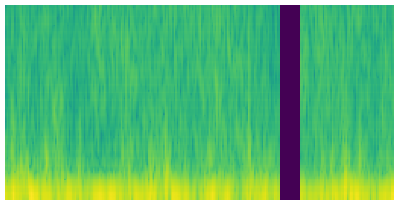
One vertical stripe (time masking) with fixed width, filled with 0
Python
params1 = {
    "num_masks_x": 1,
    "mask_x_length": 20,
    "fill_value": 0,

}
transform1 = A.Compose([A.XYMasking(**params1, p=1)])
visualize(transform1(image=img[:, :, 0])["image"])

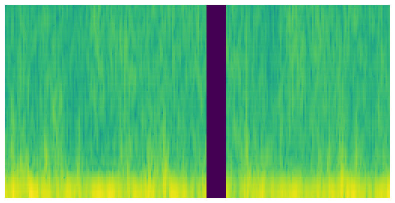
One vertical stripe (time masking) with randomly sampled width, filled with 0
Python
params2 = {
    "num_masks_x": 1,
    "mask_x_length": (0, 20), # This line changed from fixed  to a range
    "fill_value": 0,
}
transform2 = A.Compose([A.XYMasking(**params2, p=1)])
visualize(transform2(image=img[:, :, 0])["image"])
Analogous transform in torchaudio¶¶
Python
spectrogram = torchaudio.transforms.Spectrogram()
masking = torchaudio.transforms.TimeMasking(time_mask_param=20)
masked = masking(torch.from_numpy(img[:, :, 0]))
visualize(masked.numpy())
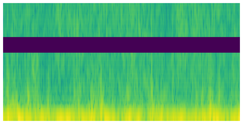
One horizontal stripe (frequency masking) with randomly sampled width, filled with 0
Python
params3 = {
    "num_masks_y": 1,
    "mask_y_length": (0, 20),
    "fill_value": 0,

}
transform3 = A.Compose([A.XYMasking(**params3, p=1)])
visualize(transform3(image=img[:, :, 0])["image"])
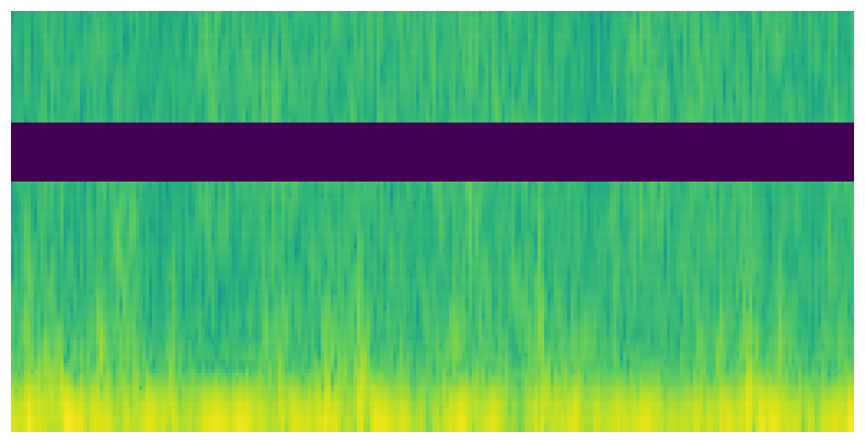
Analogous transform in torchaudio
Python
spectrogram = torchaudio.transforms.Spectrogram()
masking = torchaudio.transforms.FrequencyMasking(freq_mask_param=20)
masked = masking(torch.from_numpy(img[:, :, 0]))
visualize(masked)
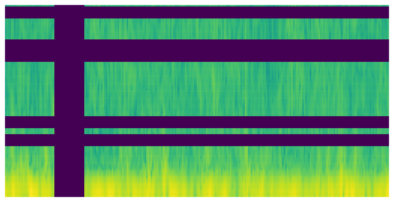
Several vertical and horizontal stripes
Python
params4 = {
    "num_masks_x": (2, 4),
    "num_masks_y": 5,
    "mask_y_length": 8,
    "mask_x_length": (10, 20),
    "fill_value": 0,

}
transform4 = A.Compose([A.XYMasking(**params4, p=1)])
visualize(transform4(image=img[:, :, 0])["image"])
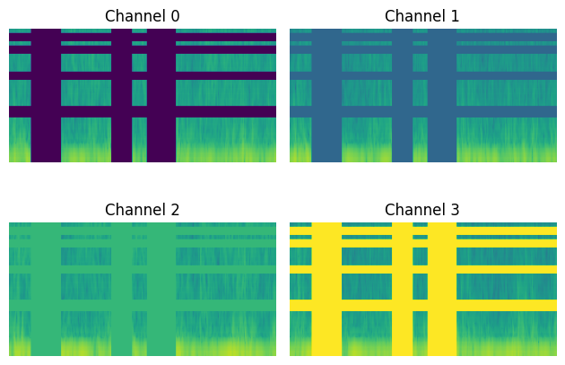
Application to the image with the number of channels larger than 3, and different fill values for different channels
Transform can work with any number of channels supporing image shapes of
- Grayscale: (height, width)
- RGB: (height, width, 3)
- Multichannel: (heigh, width, num_channels)
For value that is used to fill masking regions you can use:
- scalar that will be applied to every channel
- list of numbers equal to the number of channels, so that every channel will have it's own filling value
Python
params5 = {
    "num_masks_x": (2, 4),
    "num_masks_y": 5,
    "mask_y_length": 8,
    "mask_x_length": (20, 30),
    "fill_value": (0, 1, 2, 3),

}
transform5 = A.Compose([A.XYMasking(**params5, p=1)])
transformed = transform5(image=img)["image"]
Python
fig, axs = plt.subplots(2, 2)
vmin=0
vmax=3

axs[0, 0].imshow(transformed[:, :, 0], vmin=vmin, vmax=vmax)
axs[0, 0].set_title('Channel 0')
axs[0, 0].axis('off')  # Hide axes for cleaner visualization

axs[0, 1].imshow(transformed[:, :, 1], vmin=vmin, vmax=vmax)
axs[0, 1].set_title('Channel 1')
axs[0, 1].axis('off')

axs[1, 0].imshow(transformed[:, :, 2], vmin=vmin, vmax=vmax)
axs[1, 0].set_title('Channel 2')
axs[1, 0].axis('off')

axs[1, 1].imshow(transformed[:, :, 3], vmin=vmin, vmax=vmax)
axs[1, 1].set_title('Channel 3')
axs[1, 1].axis('off')

plt.tight_layout()

plt.show()